04 / Computational design study
Less vibration.
Enough room
to move.
A UAV payload-mount study that asks two questions together: how much vibration reaches a sensor, and how far does its mounting plate need to move?
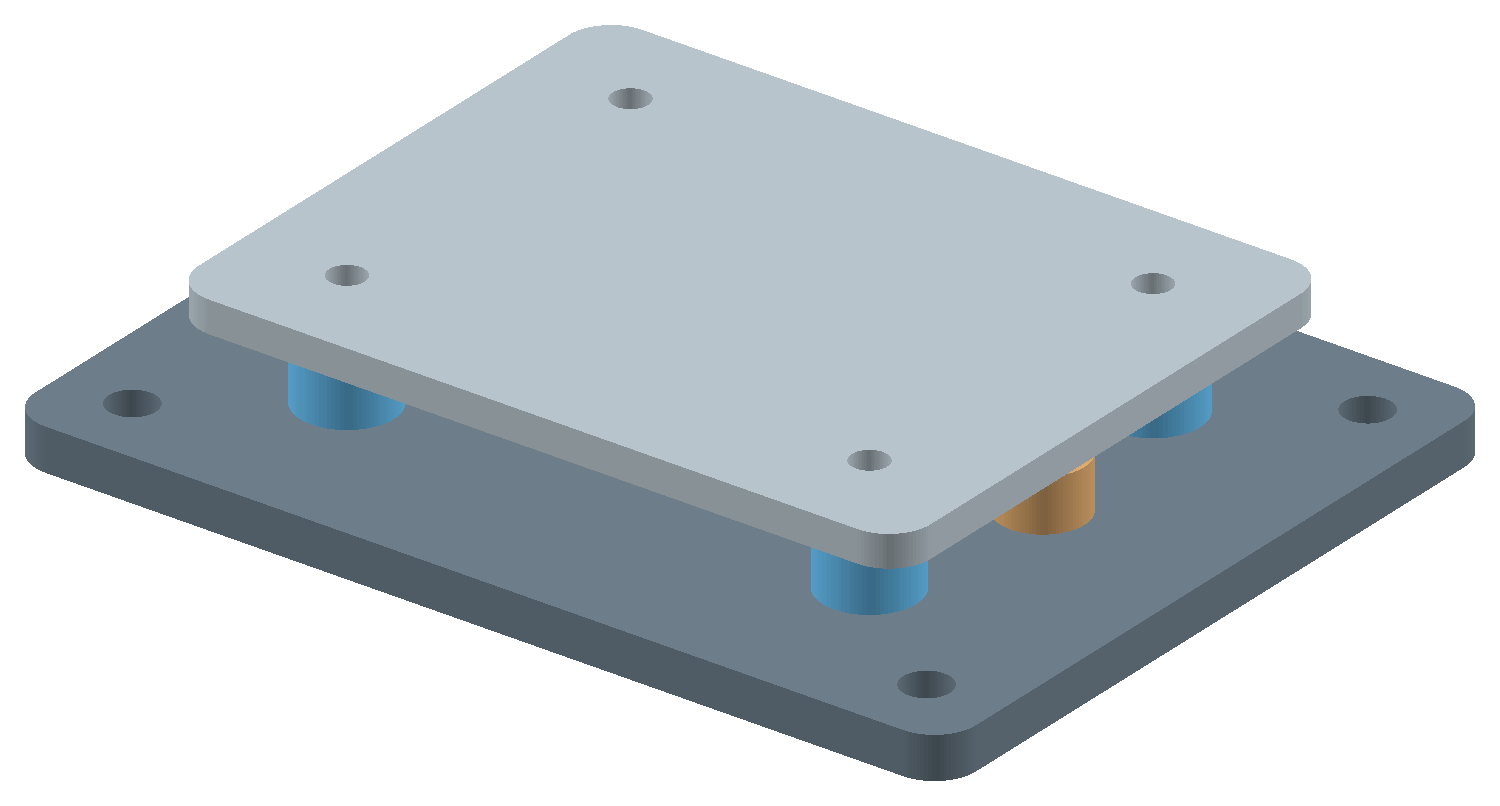 4 PARALLEL ISOLATORSGeneric geometry · assumed linear properties3.0 mmUnloaded lower-stop gap
AI-assisted computational prototype · No hardware testing
Balanced candidate, tolerance grid
Isolation needs a travel budget.
The softest mount is not the best choice.
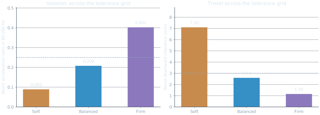
A soft mount isolates well at higher frequencies, but it uses more travel near resonance. A firmer mount controls movement, yet can transmit too much vibration. In this assumed scenario, the middle-stiffness Balanced candidate is the only one that meets both limits throughout the tolerance grid.
| Candidate | Worst ratio Limit ≤ 0.250 | Required clearance Limit ≤ 3.00 mm | Both limits met |
|---|---|---|---|
| Soft | 0.089 | 7.10 mm | 270 / 729 |
| Balanced Candidate to test | 0.208 | 2.60 mm | 729 / 729 |
| Firm | 0.402 | 1.16 mm | 505 / 729 |
Each frequency maximum includes band endpoints and any analytic stationary point inside the band. Worst isolation and worst travel can occur in different parameter combinations. Pass counts describe a deterministic grid, not a reliability probability.
02 / Interactive model
Change a choice.
See the consequence.
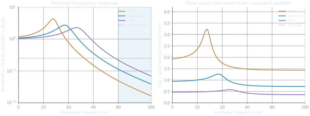
Explore a single simulated parameter set. The curve shows the response across frequency; the checks evaluate both full design bands. These live checks do not rerun the tolerance grid.
Fixed input: 0.3 g peak
Fixed unloaded stop gap: 3.0 mm
Four parallel isolators · vertical motion
Calculated values use the linear model and scenario assumptions below.
Assumptions you can inspect.
Keep the model simple enough to check.
The payload and moving plate become one rigid mass. Four identical vertical isolators act in parallel. The model describes small motion about static equilibrium; gravity sag is added separately when checking the lower stop.
m z″ + c z′ + k z = −m y″z = payload motion relative to the base · y = base motion
k = four isolators’ combined stiffness · c = total viscous damping
| Total moving mass | 0.35 kg nominal; 0.25–0.45 kg tolerance range. Includes the carried plate. |
|---|---|
| Base input | 0.3 g peak harmonic acceleration at each frequency, evaluated separately. |
| Sweep and isolation band | 5–200 Hz sweep; acceleration ratio ≤ 0.25 throughout 80–200 Hz. |
| Travel constraint | Gravity sag + peak relative motion ≤ 3.0 mm, measured from the unloaded position. |
| Parameter variation | 9 mass × 9 stiffness × 9 damping values per candidate; stiffness ±20%, damping ratio 60–140% of nominal. |
Equations, peak locations and model limits
Natural frequency: ωₙ = √(k/m), fₙ = ωₙ/(2π). Damping: c = 2ζ√(km). With r = f/fₙ, the acceleration ratio is √[(1 + (2ζr)²) / ((1 − r²)² + (2ζr)²)]. Relative peak motion is A / √[(ωₙ² − ω²)² + (2ζωₙω)²]. Static sag is mg/k.
For constant acceleration input and ζ < 1/√2, peak relative motion occurs at fₙ√(1 − 2ζ²), if this falls inside the sweep. The transmissibility stationary point is also checked, alongside the frequency endpoints.
The model excludes rocking, plate flexibility, nonlinear elastomer response, preload effects, temperature, cable bypass paths and real vehicle spectra. It does not calculate stop impacts. A predicted clearance above 3 mm fails the screening check; the no-contact solution no longer describes the subsequent motion.
Model reference: MIT OpenCourseWare, Engineering Dynamics, Problem Set 10, Problem 2 . The report includes the full definitions and primary references.
From the model to a layout.
The clearance has a physical reference.
The packaging concept places a 70 × 55 mm moving plate above a 90 × 70 mm base, with four isolators and two lower stops. The 3 mm gap is measured before gravity sag. Calling out that reference prevents a favorable calculation from hiding an interference problem.
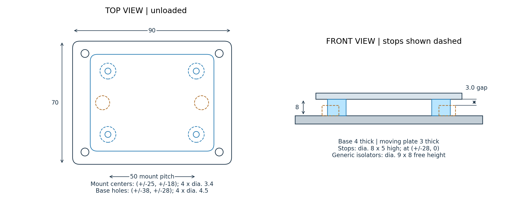
At an assumed aluminum density of 2,700 kg/m³, the moving plate is approximately 30.8 g. That mass is already included in the 0.35 kg nominal total. The isolators are generic geometric placeholders; their diameter and height do not establish the assumed stiffness.
Further work includes real isolator selection, fasteners and preload, joint loads, structural checks, manufacturing tolerances, cable routing and assembly access. This is a concept model, not a released drawing or flight-ready component.
Check before interpreting.
Numerical agreement is a check, not a test result.
A separate time-domain integration starts from rest, lets the transient decay, and fits eight settled cycles. Its acceleration and relative-motion amplitudes agree with the closed-form model to within 0.00002% at four check frequencies.
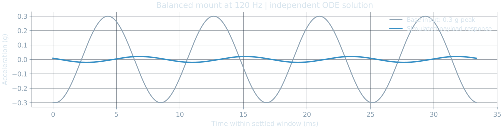
Independent integration
SciPy DOP853 at 10 Hz, natural frequency, 80 Hz and 120 Hz. Both relative travel and absolute acceleration are compared.
Dense-sweep comparison
36 checks against 100,001-point frequency sweeps, plus known response identities and static force balance.
STEP round trip
8 valid solids after re-import, volume preservation, a 3.0 mm unloaded gap and no interference above the stated numerical tolerance.
These checks verify the implementation under the same assumptions. They do not establish how an actual mount behaves. The next useful evidence is a measured load-deflection curve and a controlled bench frequency-response test.
Proposed bench validation sequence
- Characterize static behavior. Measure load-deflection and hysteresis; record loaded and unloaded stop clearance.
- Define the measurement chain. Instrument the base and carried plate; document calibration, sample rate, anti-alias filtering, fixture behavior and uncertainty.
- Approach resonance at low input. With a suitable rig and lab supervision, use stepped sine tests with controlled stop criteria before increasing amplitude. Measure relative motion directly.
- Compare, repeat and revise. Record amplitude and phase, run at least three repeats, and investigate cable stiffness, rocking, nonlinearity and temperature sensitivity.
This sequence is proposed. No physical assembly, shaker test or flight test has been performed.
A project you can reproduce.
Open the files. Follow the calculation.
The bundle contains the model, configuration, CAD source, verification code, figures, CSV results and report generator. A learning guide walks through hand calculations and a new design variation, with a log for recording work personally completed.
Authorship and current status
A transparent starting point.
AI generated the initial code, CAD concept and documentation. The outputs here come from executing that code. Personal review, independent reruns, CAD revisions and physical testing are the next steps; this version does not claim those activities have already been completed by me.
The baseline assumptions and executed checks are preserved in the source. Future contributions should be recorded with the actual changes and evidence.
Computed study version 1.0 · 22 October 2026. Primary references: MIT OpenCourseWare Engineering Dynamics; official SciPy solve_ivp and CadQuery export documentation. Full citations, environment versions, assumptions and provenance are included in the downloadable report and source.